Volume 3: Comparing Dose-Response Curves

Comparing Dose-Response Curves

Last week we highlighted that when calculating relative potency, the entire curve from the current test batch must be compared to that of the reference material, which represents batches used during clinical trials.

Occasionally, questions arise about the necessity to evaluate the full curves each time.

FasTrain Course Registration

Why Full Curve Comparison Matters

Biologically, complex molecules such as antibodies, vaccines, and large proteins can produce a range of related but basically different biological responses.

For example, an antibody may retain its ability to bind an antigen but exhibit a different affinity. Thus, appropriate binding at a given concentration may occur in the test batch, yet the binding slope could vary significantly.

This variation implies that the therapeutic concentration received by patients may in fact have a radically different potency from those administered during clinical trials.

Furthermore, as previously demonstrated, when the Test Material (TM) slope diverges from that of the Reference Material (RM), measured potency becomes dependent on the TM concentration selected for testing, rendering the assay unsuitable.

Can We Just “Eyeball” the Slopes?

How do we determine if two slopes are similar or similar enough to allow quantitation?

The simplest approach would be to have a subject matter expert, the analyst with lots of experience, look at the two slopes and make a call.

Imagine your Quality Assurance (QA) group if you proposed this approach!

Clearly we need an approach which would give us the same call regardless of who our subject matter expert (SME) is.

Model-Based Comparison Approach

To determine whether two slopes are sufficiently similar to accurately measure potency, a common practice involves fitting experimental data to models such as the four-parameter logistic (4PL) curve or, in some cases, a two-parameter linear (2PL) model. (This is a straight line).

These fitted models facilitate objective comparisons of slopes rather than relying solely on expert judgment.

For illustration, consider a published example comparing a WHO reference standard for a vaccine to a test batch. The complete details will not be covered here; further information is available at www.fastraincourses.com through the Potency Bioassays: Development and Validation Training Course.

However, here is the Cliff Notes version of the approach.

Step 1: Fit Individual Curves

Step 1: Fit a 4PL curve to individual RM and TM samples. This is called the Best Fit Curve.

Step 2: Compare Slopes

Step 2: Determine if the ratio of the slopes falls within an empirically established acceptable range.

The range is often established by running two RM samples within a single assay and comparing RM1 Slope/RM2 Slope.

In the provided example, the slope ratio is 0.65/0.83 = 0.78, and the acceptable range for this assay was set at 0.75–1.25.

Therefore, the slopes are considered similar.

Step 3: Establish a Consensus Curve

Once similarity is established, potency calculation follows.

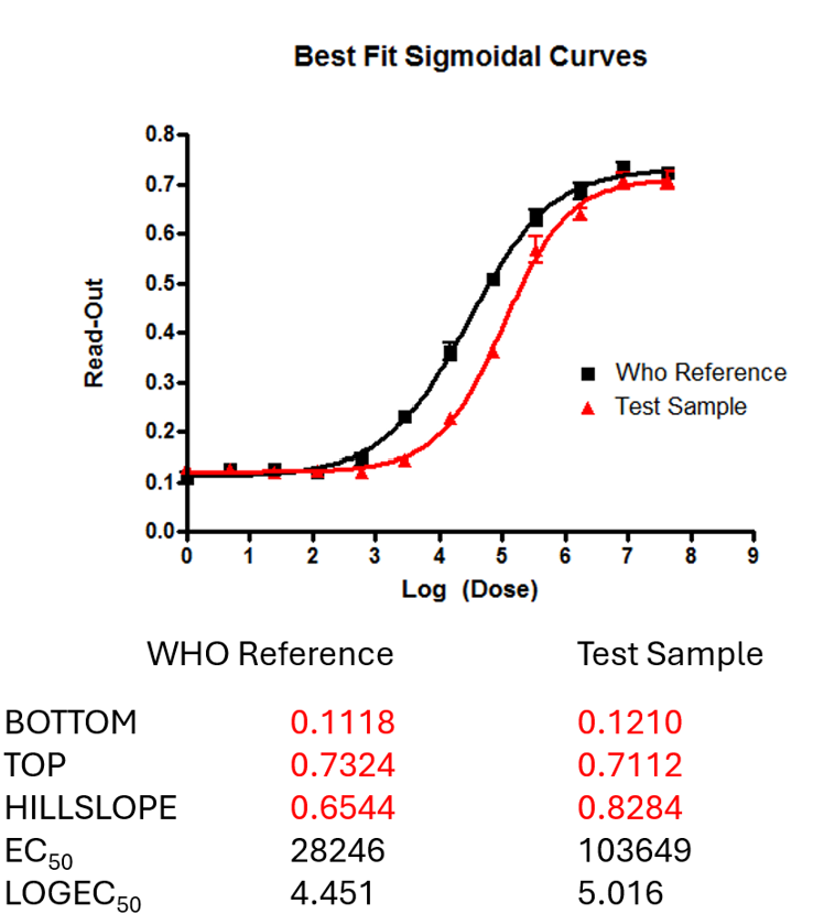
The concentration ratio required to achieve a 50% response (EC50) for both batches is evaluated.

It is important to note that even with similar slopes, slight differences can affect potency estimates depending on which response level is chosen (e.g., 50%, 45%, 70%).

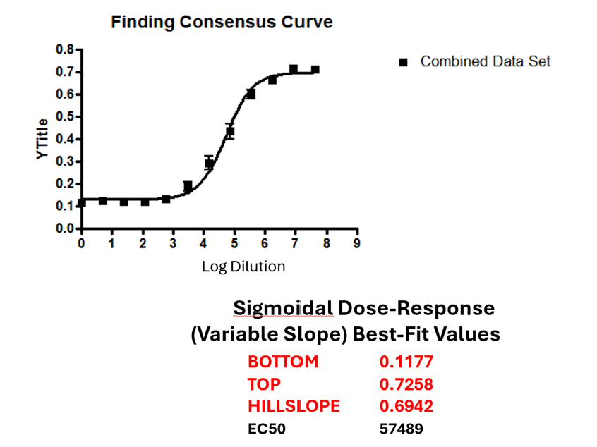
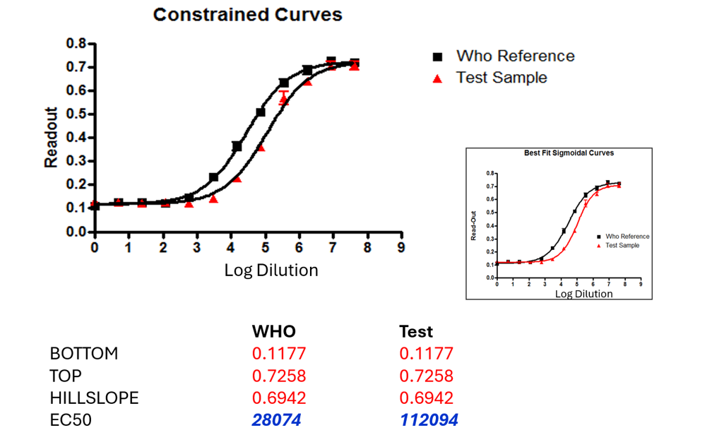
To address this, a “consensus” (sometimes referred to as “constrained”) slope is calculated using all data combined as if they originated from a single sample set.

The resultant best-fit curve of this combined dataset produces the consensus slope.

So, Step 3: Establish the consensus curve fit using the entire dataset.

*The same data set is used below as in the above graph.*

Notice the newly calculated consensus slope is, as expected, some value between the two slopes for the best curves of the individual datasets shown above.

The consensus slope is 0.69.

Step 4: Refit Using the Consensus Slope

Step 4: Refit individual RM and TM samples utilizing the consensus slope.

Applying this approach yields updated fits for the dataset.

Step 5: Final Potency Calculation

Step 5: The final step involves potency calculation using the EC50 values for TM and RM:

Potency = 112094 / 28074 = 399.3

Software Considerations

There are numerous software packages available (including PLA from Stegmann Systems, Softmax Pro, Unistat, Statlia, among others), each implementing distinct algorithms to derive statistically robust estimates.

Comparative analyses indicate consistent potency outcomes across platforms, allowing users to select software best suited to their requirements.

Have Questions?

This is an interactive newsletter!

We want to hear your burning bioassay questions.

Send your questions to Dr. Laureen Little (laureen.little@fastraincourses.com) and she and our team of instructors will answer them in the coming newsletters.

Laureen's Email for Questions

If you ever miss a volume or want to revisit key points from previous issues, we will be updating the Bioassay Month page throughout the series.

Bioassay Month Updates

Interested in FasTrain Bioassay Courses?

Explore the full list of bioassay courses we offer.

Potency Bioassays Development & Validation

CMC Relative Potency Analytical Methods: A Technical Deep Dive

Introduction to Statistics for Potency Bioassays

Statistical Method in Bioassay

Cell Culture and Cell-Based Assays

Course Registration